Even though many teams use established tools like Jira or Rally to track work in progress (WIP), capturing the raw data yourself is worthwhile. Knowledge is power, after all – once you have the data, you can generate visualisations to help you interpret your WIP, Throughput, Cycle Time and other useful metrics.

In this blog series, I’ll be showing you how. In this first part, I’ll run through a step-by-step guide on how to create a spreadsheet that helps you capture and visualise data about your team’s process. In the posts that follow, I’ll show you how to make it start working for you.

Assumptions

The key assumption made in this post is that your team’s process has six stages: To Do, Analysis, Ready, In Progress, Demo Ready, and Done.

Of course, your team’s process is unlikely to exactly match the one in my example, so I’ll state when you need to swap out the example for your own data. You might want to run through this example first for clarity.

Oh, one more thing – the example in this post uses a Google Docs spreadsheet, but it will work just as well in Microsoft Excel.

Let’s get to it.

Creating your spreadsheet

1) Create a new spreadsheet and rename ‘Sheet1’ to ‘Data’

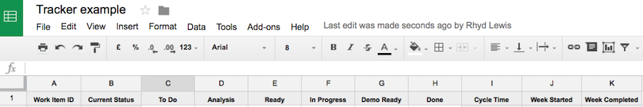
2) Add the following header columns (starting in cell A1). If you’re using your own process, just add or remove columns as needed.

A	B	C	D	E	F	G	H	I	J	K
Work Item ID	Current Status	To Do	Analysis	Ready	In Progress	Demo Ready	Done	Cycle Time	Week Started	Week Completed

 

Here it is in a Google sheet:

 

3) Copy and paste these formulas into the appropriate cells:

Cell	Calculation	Formula	Note
B2	Current Status	=INDEX($C$1:$H$1,1,COUNTA(C2:H2))	Shows a work item’s current status. Useful when comparing against the team’s board.
I2	Cycle Time	=IF(ISBLANK(H2),””,NETWORKDAYS(C2,H2))	Determines the number of elapsed working days between work starting (To Do) and finishing (Done).
J2	Week Started	=IF(ISBLANK(C2),””,C2-WEEKDAY(C2,2)+1)	Calculates the week in which work started.
K2	Week Completed	=IF(ISBLANK(H2),””,H2-WEEKDAY(H2,2)+1)	Calculates the week in which work ended.

 

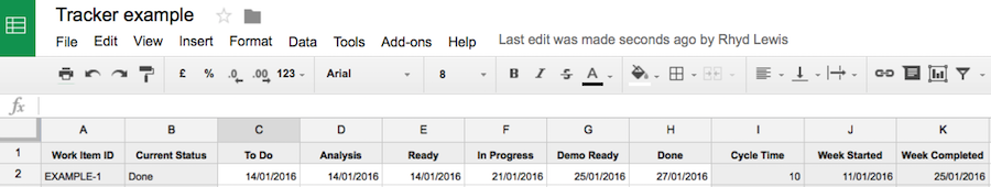
You’ll have something like this:

 

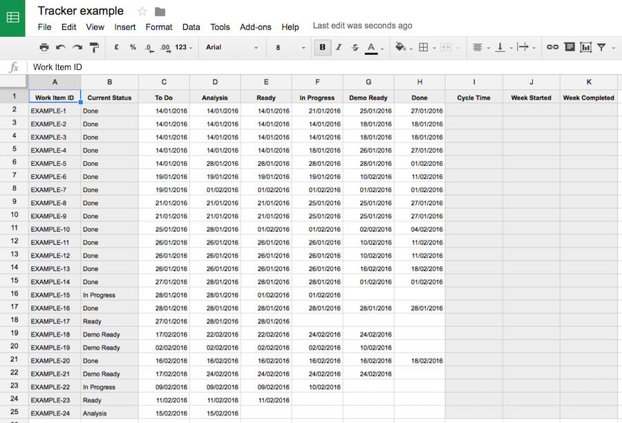
4) Simple, right? Now let’s add some test data into the sheet to show how it works.

 

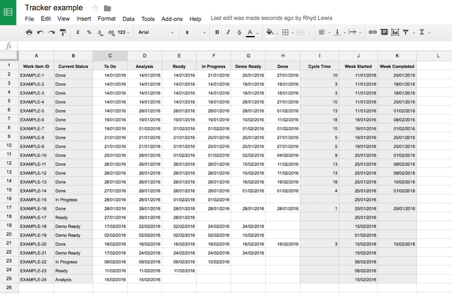
5) Now copy/fill down the formulas you entered in columns B, I, J and K down each column, until you reach the end of the test data. This will update the calculated data like so:

 

The key activity to make this tracker useful is to capture the date on which a work item changes state. For example, if your team moves a work item into the ‘To Do’ column on 19/01/2016, enter that date in the ‘To Do’ column in your tracker. When the team moves the work item into In Progress on 21/01/2016, enter that date into the tracker column named ‘In Progress’.

Staying up to date is simple

Capturing the raw data will only take a minute or two each day, whether your team uses a physical board or an electronic one. I’ve found the approach that works best for me is to update the tracker with changes from the team board after stand-up. For work items that have:

• moved forwards: add today’s date into the appropriate status column. If it’s moved by more than one column, put today’s date in the skipped columns too.
• moved backwards: delete any date captured beyond what is now the current state.

You now have your spreadsheet ready! Keep an eye out for part two, when we’ll start looking at what to do with the data. If you can’t wait, I can recommend Dan Vacanti’s book Actionable Agile Metrics for Predictability for those interested in further reading on this subject.